Research Article 
![]() Creative Commons, CC-BY
Creative Commons, CC-BY
On The Closed Trajectory of Movement of Biological Time Inside the Organism of a Plant in Ontogenesis and Everything Secret Becomes Apparent
*Corresponding author:Naumov Mikhail Makarovich, Department of ecological and hydrometeorological, University State Ecological Odessa, Ukraine.
Received: March 22, 2022; Published:March 28, 2022
DOI: 10.34297/AJBSR.2022.15.002176
Abstract
The work considers a separate biological time in plant ontogenesis. Based on the proven method of degree - days, the sum of scalar products of two-time vectors of biological time is built. Further, a curvilinear integral of the second kind is found as a replacement for the degree-day’s method. An open curvilinear integral only shows the assumptions about the properties of time inside the plant organism. A closed curvilinear integral of the second kind fully proves the assumption made: time inside the plant’s organism is closed. The conclusion is made about the existence of a temporary surface inside the plant organism. Biological time is compared with the influence on the movement of chromosomal material inside the cell. It turns out that the chromosome is completely subordinated to biological time, or simply time. All calculations are based on the material processes of photosynthesis, respiration, plant growth in ontogenesis.
Introduction
In this work, we will consider time. We can consider time only by the totality of material processes that occur inside the plant’s organism. We will distinguish between biological and physical time. Biological time has the property, inside the plant organism, to stretch or shrink depending on the weather, from the state of agrometeorological factors (this was established by Reaumur in the XVIIIth century). So, it has long been established that the rate of development of a plant organism depends primarily on the ambient temperature [1]. Subsequently, practical data were obtained that indicate that the rate of development of plants depends on such agrometeorological factors as their state at the current moment of growth and development: light - the arrival of FAR [2,3,4] moisture - reserves of productive moisture in the soil [2,3] nutrition - mineral nutrition in the soil-NPK [5]. These factors, together with the properties of physical time and our three-dimensional physical space, are the basic component of a plant’s organism for life. In this work, we will show, at least, that the biological time of a plant moves along a closed trajectory and determines the growth of dry biomass of the plant’s general organism.
Materials and research methods
Change in biological time on a straight time axis
We will assume that there is its own biological time inside
the plant organism. As soon as we assumed this, we immediately
receive in response a method for calculating this biological time
of a plant: this method consists in the fact that for each day of
ontogenesis, the relative values of the increments of dry biomass
of the whole organism of an annual plant and changes in the
increment of biological time under different agrometeorological
factors are compared, and the same moment of ontogenesis [6].
I have shown that the calculation of the biological time of a oneyear
plant organism until the moment of the “flowering” phase
can be obtained by the equation T (j+1) = T0 +T ( j) + ΔToptΩ(j)
,T0< T(j) < 0,5, (1) where T0 - the initial value of the biological
time corresponding to the “shoots “phase of an agricultural crop
(or simply a plant), relative units; T(j) - is the current value of
the biological time of the whole plant organism for the lived day
j, relative units; Δ Topt - is the increase in biological time for one
calculated day of plant growth and development with optimal
agrometeorological factors, relative units; Ω (j) - the normalized
value of CO2 gas exchange in the whole plant organism, which is the
value of CO2 gas exchange at low agrometeorological factors, divided
by the amount of CO2 gas exchange at optimal agrometeorological
factors of the whole plant organism as a whole in one calculated
day, relative units. The “flowering” phase itself determines new
essential physiological properties in the plant. After “flowering”
changes occur in the growth and development of the plant. So, in
sunflower and other crops, the growth of leaves, stems, petioles, and
roots stops. At the same time, after the flowering of the sunflower,
the processes of dying off all vegetative organs begin to occur and
only the generative organs continue their growth and development.
When the vegetative organs die off, part of the biologically active
substance from the vegetative organ is sent to the generative organs
- the basket and seeds, the rest of the vegetative organs simply ends
their growth and development. Therefore, the calculation of the
biological time of a plant changes significantly after the “flowering”
phase [6]. Thus, after the “flowering” phase, before the “maturation”
phase, the calculation of the biological time can be carried out
according to the equation T(j+1)=T(j)+ΔTopt/Ω(j),0,5
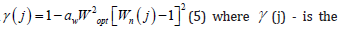
These two equations (1) and (2), allow calculating and making predictions of the onset of flowering and full maturation phases, depending on the current agrometeorological factors, as a simple sum for each day of plant life on an accrual basis. Other phases of plant development can be found as additional biological times for each phase of plant development. At the same time, these values of biological time will be located only in the middle of the interval from Т0 to 1. (For sunflower, these may be the following additional vegetative phases: “real third leaf”, “budding”, “milk ripeness”, “wax ripeness”, for other crops, other corresponding vegetative phases of development). For such a calculation, for the implementation of the forecast, before the date of the forecasts, real data are taken on the agrometeorological factor that already existed during the life of the plants. And the missing future agrometeorological factors can be taken as mean long-term values, or, according to longterm meteorological forecasts. As soon as the required number of biological times has come, the calculations are stopped. The value of the correction Ω (j) of the optimal value of the increase in biological time for the current state of agrometeorological factors, in the first approximation for sunflower, can be calculated as a simple product of the normalized value of the light curve of photosynthesis [9,10] the normalized temperature curve of photosynthesis [10] the normalized wet curve moistness soil influence of photosynthesis [11] the normalized curve of the mineral nutrition of plants [12]. All normalizations of the curves are given by me according to the corresponding curves from their maximum value. The normalized lights curve of sunflower for the FAR flow is as follows I (j) = 1− exp[−CIoptIn(j)] , (3) where I(j) - is the normalized value of the lights curve influence of sunflower photosynthesis, relative units, varies from 0 to 1, it is assumed that the exponent has its maximum; С - parameter, m2·W-1; Iopt - is the value of the FAR flux at which the maximum intensity of photosynthesis is observed, W·m2; In(j) - the normalized value of the real FAR flux coming to the upper sowing border, is found as the current FAR flux value divided by the FAR flux value in a cloudless sky, relative units. The temperature curve for the influence the intensity of the photosynthesis process has the form ψ(j)=1-att2opt[tn(j)-1]2 (4) where ψ (j) - is the current normalized value of the temperature curve of the intensity of the photosynthesis process, varies from 0 to 1, relative units; at - parameter, (CO)-2; topt - is the optimum air temperature for the intensity of the photosynthesis process, Co; tn(j) - the current normalized value of the air temperature inside the crop, relative units, is found as the value of the air temperature divided by the temperature at which the maximum intensity of the photosynthesis process is observed. The soil moisture curve of the intensity of the sunflower photosynthesis process has the form
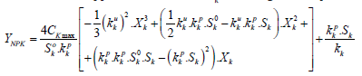
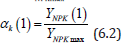
(6.1) where YNPK - the value of the total yield of dry biomass of a plant, depending on the applied dose of fertilizer, 100·kg·ha-1; Ckmax - constant, parameter, rate of increase in total dry biomass depending on the unit of increment of the fertilizer dose Δ Ymax· Δ Xk-1=Ckmax , kg·kg-1; kk - is the content of the k-th nutrient per unit all dry biomass of the gathering in of the crop, rel. units. Such a calculation, according to equation (6.1) the value of dry biomass will not be accurate, since the crop yield depends on the prevailing agrometeorological conditions of plant life. To exclude this property of equation (6.1) it is necessary to make another calculation of the value of the total dry biomass of the crop according to equation (6.1) but at the value of the maximum fertilizer dose, which was obtained earlier according to equation (6). Finally, the effect of the applied dose of fertilizer on the rate of growth and development of the crop[12] can be obtained as the ratio of the yield value, taking into account the applied dose of fertilizer YNPK, obtained according to equation (6.1) to the value of the maximum yield YNPKmax, obtained from equation (6.1) according to the equation
Results of calculating biological time on a straight time axis
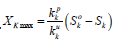
The onset of phenological phases of flowering and maturation of sunflower for years different in agrometeorological conditions are given in (Table 1). As can be seen from (Table 1), the dates of the onset of vegetative phases of development almost completely coincide with the calculated data. The difference in the duration of the between-phase periods can be ensured by the accuracy of the calculations and by the fact that several agrometeorological stations were taken for the dates of the onset of the “flowering” and “maturation” phases. In total, 7 agrometeorological stations located on the territory of the Odessa region were processed for calculations. (Table 1). As can be seen from the data obtained in the calculations of the phase “flowering” of sunflower occurs on average 63 days after “shoots”. At the same time, these 63 days correspond to the value of the biological time axis equal to 0.5 relative unit’s timeline. The “maturation” phase on average, in the calculations, is 103 days from the “shoots”, which is a fairly accurate calculation, and the value of the biological time axis is 1.0 relative units. It should also be noted that the calculation equations (1) and (2) use the same value of the optimal increase in biological time Δ topt, both before “flowering” and after “flowering”. This means that the biological time moves inside the plant organism unambiguously, both before flowering and after flowering and is determined only agrometeorological factors of life. So, we got that over biological time varies depending on the weather changes, agrometeorological conditions depending on changes in gas exchange of CO2 the whole body of the plant. At the same time, the calculation is carried out for one day of plant growth for the entire ontogenesis. For each culture or crops variety is its value of quantity Δ Тopt.

Figure 1: Influence of different doses of nitrogen N and different doses of the optimal value of nitrogen content N in the soil, as an active substance, on the yield of dry total biomass of winter wheat: YN - yield of total dry biomass, 100·kg∙hectare-1. XN - is the value of the applied nitrogen dose, kg active substance∙hectare-1. S0N - different values of the optimal nitrogen content in the topsoil 0-20 cm, kg active substance∙hectare-1. units of measurement - YN, kg·ha-1

Table 1.Comparison of the calculated and actual dates of the onset of the phenological phases of sunflower development for different years on average for the whole Odessa region (actual data obtained by the Hydrometeorological Service of Ukraine).
Biological time as an unclosed curvilinear integral of the second kind
It should be noted the following fact of the already proven change in the movement of biological time calculated by equations (1) and (2). So, if we consider changes in the increments of biological time, then this increment becomes depending on agrometeorological conditions on each day of plant growth and development. This means that we can assume that the vector of the maximum in biological time Δ Topt deviates from its direction in the plant. And we can think of the modified vector ΔT as the dot product of two vectors. In this case, as we believe, the deviation of the vector Δ Topt occurs from the axis of physical time, which flows in its own way. Then the projection of the deflected vector Δ Topt onto the direction of the physical time axis will give the values of the vector Δ T. That is, we can consider the scalar product of two vectors: 1. The vector Δ Topt, deviated from the physical axis of time t, and 2. The vector Δ Topt lying on the axis of physical time t. Thus, we follow the fact that during the life of a plant, we need to find the sum of the scalar products of two vectors of the biological time of the plant according to equations (1) and (2). Such a calculation was made, and we can see the change in the biological time axis in relation to the change in the physical time axis in (Figure 2). As can be seen from (Figure 2) biological time is significantly changed in relation to physical time. At the same time, it is necessary to immediately note the following fact: we consider the scalar product of two vectors, then the first vector can deviate from the physical axis of time only in the two-dimensional time space inside the plant organism. For further calculations, we need to make some assumptions: we will consider the fact that in the whole ontogeny of a plant, the process of photosynthesis and the process of respiration change from day to day, smoothly. That is, they are smooth curves. The same can be said for the two-time axes - they are smooth curves. Then we can proceed to consider our phenomenon in a differential form.

Figure 2: Change in the flow of biological time in relation to physical time, Odessa, settlement “Chernomorka»: 1 - average long-term values of agrometeorological factors;2 - agrometeorological factors of 1986 of the year; 3 - agrometeorological factors of 1987 of the year. units of measurement – T(j), relative units
Then, the growth of the total dry biomass of the whole plant organism follows a smooth S - shaped curve. To begin this consideration, we write down an open curvilinear integral of the second kind, which fully corresponds to equations (1) and (2).
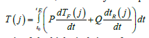
(8) here T(j) - is the summed axis of the biological time of an annual plant; P -some function; - rate of change of the first axis of biological time; Q - some function; - the rate of change of the second axis of biological time; t0- initial integration physical time, corresponds to the “shoots” phase; tE - the final integration physical time, corresponds to the “maturation” vegetative phase; t - is physical time. In equation (8) it immediately follows that we are considering the process of biological time of a plant already in two-dimensional time space. This also follows from equations (1) and (2). It is advisable when considering equation (8) to use the material processes of photosynthesis, respiration, growth rate. Let us now consider the fundamental equation for the growth of the total dry biomass of a plant, obtained by [14] of the year. , dMdm/=dt dFdm/dt-dRdm/dt (9) where dMdm/dt - is the growthrate of the total dry biomass of the whole plant, gdm·days-1; dFdm/ dt - process (rate) of photosynthesis of the whole plant organism expressed in dry biomass, gdm·days-1; dRdm/ dt - the process (rate) of respiration of the whole plant organism, the costs of the respiration process are also expressed in dry biomass, gdm·days-1; dt - is the differential of physical time, in the case of this equation it is one day. This equation shows that the increase in the total dry biomass of the whole plant organism is determined by the rate of CO2 gas exchange of the entire plant. For a practical view of the increments in the total dry biomass of potatoes during the entire ontogenesis, see (Figure3). Also, this (Figure 3) gives direct views on the magnitude of the change in the process of photosynthesis and the process of respiration in plant ontogenesis according to equation (9). In addition, as can be seen from (Figure 3), for each year of observation there is its own, different, maximum growth rate of the total dry potato biomass. This is ensured by years of different weather conditions. dM/dt, gdm·m-2·days-1 physical time, day from “shoots”. To compare the integrand of equation (8) with the equation for the increase in total dry biomass (9) we need to find the normalized values of the increase in total dry biomass during ontogenesis. This must be done because the biological time of a plant is also expressed in relative units. To do this, consider the sigmoid curve of plant growth, (Figure 4), and normalize it to the value of the final total dry biomass of the whole plant organism. In this case, the sigmoid curve grows of the plant will change from some small μ0, corresponding to the «shoots» phase, to one. Corresponding to the “maturation” phase, and in years different in weather conditions will have almost the same appearance, depending on in the movements of the biological time of the plant. Then we can write
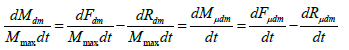
(10) where Mmax - is the value of the total dry biomass of the whole plant organism for the “maturation” phase, this is the maximum value of the total dry biomass of the plant, gdm; dMμdm - is the normalized value of the increments (differential) of the total dry biomass of the whole plant organism, relative units·day-1; dFμdm - normalized value of increments (differential) of total dry biomass in the process of photosynthesis, relative units·day-1; dRμdm - is the normalized value (differential) of the costs for the respiration process of the whole plant organism, relative units·day-1. Now we can compare equation (8) - its integrand, with the equation of Davidson J.L. and Philip J.R.
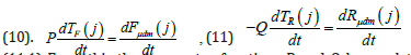
(11.1) From this the two vector functions P and Q have relative units in their dimension. The value of these two vector functions P and Q can be a value equal to one. Then the rate of flow of biological time in relation to physical time for the processes of photosynthesis and the process of respiration will be different. So, the speed of movement of biological time for the process of photosynthesis will be completely positive, and for the process of plant respiration - negative. This conclusion, moreover, follows from the fact that in the process of photosynthesis there is a positive increment of new biomass substance, and in the process of plant respiration, the created biomass is consumed from the plant organism and energy is generated for growth. Thus, in the process of plant respiration, biological time (or simply time) moves backward. Let us now write down the complete non-closed curvilinear integral of the second kind for calculating the processes of the flow of biological
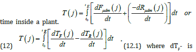
(12.1) where dTF- is the rate of flow of biological time corresponding to the process of photosynthesis, relative units·day-1; dTR- the rate of flow of biological time corresponding to the respiration process, relative units·day-1. For calculations according to equation (12), we need to know the functional dependence of the processes of photosynthesis and respiration in ontogenesis in the form of a mathematical expression. But we can do without it since the processes of photosynthesis and respiration determine the increase in dry total biomass. Therefore, equation (12) is nothing more than a sigmoid plant growth curve expressed in relative units. That is, we believe that the movement of biological time is of the basics function of the processes of photosynthesis, respiration, and growth.

Figure 3: Increases in the total dry biomass of potatoes per square meter of soil surface during ontogenesis in different years, according to Tooming H.G. – 1984. units of measurement — dM/dt, gdm·m-2·days-1

Figure 4: Sigmoid growth curve of total dry biomass of sunflower per square meter of soil surface: 1 — 1986 the yars; 2 -1987 the yars. biological time, day.
The biological time of a plant organism as a closed curvilinear integral
It is well known that crops such as sunflower, spring and winter wheat, barley and others begin their life cycle from a seed, and this life cycle continues until new seeds appear in the plant’s organisms. That is, there is a movement of life from “seed” to “seed”. In addition, the process of photosynthesis, its growth for the entire dry biomass during the day, starts from zero (we believe that there is no photosynthesis in the seed) and, passing its maximum during ontogenesis, again comes to zero (the growth processes at the time of maturation have stopped). More difficult with the respiration process. - We believe that the material process of respiration all the time occurs in the seeds of a plant as a basic component of life. Therefore, the process of respiration of the whole plant begins with a certain small value, passes a maximum during ontogenesis, and ends again with its small value. All this allows us to speak about the closedness of biological time inside the plant organism as a property that determines the basic component of plant life, and makes the plant follow from the beginning of life “seed” to the end of life again “seed”. That is, inside the plant organism, the movement of biological time is carried out along a closed trajectory. This trajectory can be very diverse for different plant species. Closed trajectory can be either with self-intersections or without self-intersections. We’ll look at one closed trajectory that goes to a sunflower plant. We will assume that in the simplest case, the closed trajectory of the movement of time inside the sunflower organism is a circle r2 = ( X −1)2 +Y 2 (13), where r - is the radius of our time circle, relative units; X - the first-time coordinate, relative units; Y - the second time coordinate, relative units; the movement of time goes clockwise. Let us show that such a material movement of biological time in the ontogenesis of a sunflower along our time circle corresponds to its processes of growth and development. Let’s write our time circle in parametric form TF(j)=1-cos(2πt(j)) (14) TR(j)=sin(2πt(j))(15) here t(j) - parameter - physical time, varies from small t0 to 1, rel. units; if t(j) is expressed in days , then it is equal to 1/tE, where tE is the duration of the entire ontogenesis, rel.units·days-1 ; TF(j) - the normalized value of the biological time corresponding to the process of photosynthesis, relative units; TR(j) - the normalized value of the biological time corresponding to the respiration process, relative units; j - is the number of the day of the billing period. By the condition of the problem of calculating the biological time circle, we consider the temporary physical points t0 and tE the closed, that is, the same time point on the circle. Now we will find the length of our time circle, where this length corresponds to the duration of time of the entire ontogenesis, according to the equation
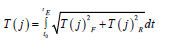
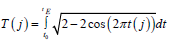
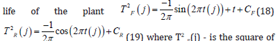
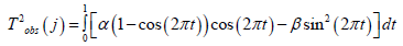
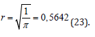

Figure 5: day of physical time from “shoots” The general movement of the biological time of sunflower during ontogenesis, obtained from its model of the production process for three years of observations, according to equation (16): SRMN – average long-term agrometeorological conditions for 1975-1999; 1986 - agrometeorological conditions 1986, station “Chernomorka”, city Odessa.

Figure 6:physical time, rel. units, 1/tE Change of the integral of biological time corresponding to the process of photosynthesis - TF, and the integral of biological time corresponding to the process of respiration — TR, during ontogenesis of an annual plant. T2obs (j) - work of a temporary force field in ontogenesis, (rel. units)2

Figure 7:physical time t, rel. units Calculation of the curvilinear integral of the 2 - nd kind for time ellipses according to the equation (21): 1 – circle:α =1/ 2;β =1/ 2; 2 - ellipse: α = 3 / 4;β =1/ 4; 3 - ellipse: α = 2 / 3;β
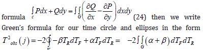
Green’s formula
Let us recall the equation that goes from a curvilinear closed contour to a double integral according to Green’s
Discussion
We began our consideration of the biological time of a plant by accepting an important fact: the biological time of a plant differs from physical time and tends to stretch or contract depending on the current state of agrometeorological factors. Then, in a natural way, we obtained the scalar product of two-time vectors for one day of calculation in plant ontogenesis, according to the proven method of degree-days (effective air temperatures) (Guide to Agrometeorological Forecasts 1984) [16]. However, the method of degree-days (sums of effective temperatures) is in no way connected with the material processes of the plant organism. Then it became necessary to establish such a connection. The method of degree - days (sums of effective temperatures) gives an unambiguous representation of it as a sum of scalar products of two-time vectors for each day of calculations. One of them is closely related to physical time and our three-dimensional space, and the second time vector is deflected from it at a certain angle in the two-dimensional time space of the plant organism. Then, to calculate biological time, it is natural to use a curvilinear integral of the second kind. This was done with the assumption that the integrand of the curvilinear integral corresponds to the material processes of photosynthesis and respiration of the plant organism. First, we calculated the temporal length of the curve corresponding to the material processes of photosynthesis and respiration. But we could not get complete confirmation of the correctness of our statements based on an open curvilinear integral. In what follows, a closed curvilinear integral over a circle is considered. And already this circle gave full confirmation of the correctness of our research. We compared the parametric equations of our time circle with the normalized values of the processes of photosynthesis and respiration in plant ontogeny and obtained an unambiguous correspondence with the processes of changes in biological time. In addition, instead of the time circle, a time ellipse is considered. With its help, it is possible to select S-shaped curves of the growth of the organism of a plant of any kind. This correspondence is expressed by the sigmoid growth curve of an annual plant. In addition, it becomes clear that the parametric equations of the biological time of a plant can be repeated at each growing season of a plant’s life, since they are expressed by trigonometric equations. In addition, the resulting integral of parametric temporal equations suggests that in the chromosomes of the seed, its cells, there is a constant value of the biological time process. Only this biological time, its process, is closed in chromosomes. This means that the seed has a living state, and when it gets into the right agrometeorological conditions (the right heat and moisture), the processes of growth and development, respiration and photosynthesis of the plant organism begin to be activated. The closed curvilinear integral of biological time is not equal to zero. This means that biological time depends on the path of its movement. And within this time domain there may be points or even some inner rip areas. Such an area of rupture can be a vacuole, where cell juice is present and there are no other components of the cell that perform cellular and organismal functions. According to Green’s formula, we have a temporary surface inside a plant’s body in its cells with a gap in the form of a vacuole. Living cells can be thought of as the additive sum of temporary surfaces in a plant organism. This easily follows from theorems on double and curvilinear integrals. At the same time, the time area on the plane can be represented as a temporary surface in a three-dimensional time space inside the plant organism, which can be projected onto a two-dimensional time plane. That is, such a statement unambiguously follows from Stokes’ mathematical formula. Moreover, such a temporary surface in three-dimensional time space can be very diverse: from a ball to an ellipsoid and other surface, it can be open. But that’s another study.
References
- Shigolev AA (1957) Temperature as a quantitative agrometeorological indicator of speed development of plants and some elements of their productivity. Proceedings of the TsIP -Vyp 53: 75-81.
- Ventskevich GZ (1960) From the experience of work on the critical processing of phenological material agrometeorological year books. Proceedings of the Central Institute of Forecasts 98: 99-108.
- Dmitrenko VP, Gatsenko RV, Lapteva NI (1989) On the quantitative assessment of the influence of the main agrometeorological factors on the duration of interphase periods of winter wheat. Proceedings Regional Research Hydrometeorological Institute. "Climate, weather and harvest" 234: 43-59
- Avksentieva OA (2007) Features of carbohydrate-protein metabolism of plants of various photoperiodic groups in connection with the reaction to the photoperiod. Bulletin of Kharkiv National university im. V N Karazin Series “Biology” Vip 5(768): 157-165.
- Avdeenko SS, Shevchenko AS (2021) Features of the growth processes of early ripe potato varieties for technical purposes, depending on the mineral nutrition in the Rostov region. Donskoy State Agrarian University.
- Naumov MM (2005) Plant growth and biological time. Bulletin of ODEKU 1: 72-78.
- Anderson WK, Smith RCG, McWiliam JR (1978) A system approach to the adaptation of sunflower to nev environments. I. Phenology and development. Field Crops Research 1: 141-152.
- Babushkin LN (1951) Assessment of the influence of weather on the rate of development of cotton and other agricultural crops and methods for predicting the onset of the main phases of their development under conditions Uzbekistan. Methodical instructions of the TsIP 16-47.
- Rabinowich E (1951) Photosynthesis and Reated Processes, Vol. II, part 1. There is a translation: Rabinovich E. (1953) Photosynthesis 2-651.
- Horie T (1977) Simulation of sunflower growth. Bull Natl Inst Agric Sci Ser A 24: 45-70
- Polevoy AN (1983) Theory and calculation of the productivity of agricultural crops. -L.: Gidrometeoizdat 175.
- Naumov MM (2006) Accounting for the level of mineral nutrition of plants in dynamic models’ production process. Bulletin of ODEKU 3: 114-123.
- Tooming HG (1984) Ecological principles of maximum crop productivity. Leningrad 264.
- Davidson JL, Philip J R (1958) Light and pasture growth. In.: Climatology and microclimatology. UNESCO 181-187.
- Naumov MM (2006) Dynamic model of sunflower production process. Meteorology and hydrology 6: 104-110.
- (1984) Manual of Agrometeorological Forecasts. Leningrad: Gidrometeoizdat 1-309.


 We use cookies to ensure you get the best experience on our website.